Replication of Sims (2010)

This example replicates Sims (2010) from the Handbook of Monetary Economics using the DRIPs package.

to run and modify the following code (no software is needed on the local machine).

See Afrouzi and Yang (2020) for background on the theory.

Setup
Initialization
Solution
Impulse Response Functions
Extensions
- Transition Dynamics of Attention
- Impulse Response Functions with Information Treatment

Setup

The problem in Sims (2011), as it appears on page 21, with slight change of notation,

\[\begin{aligned} & \min_{\{\Sigma_{t|t}\succeq 0\}_{t\geq 0}} \mathbb{E}_0\left[\sum_{t=0}^\infty \beta^t \left(tr(\Sigma_{t|t}\mathbf{H}\mathbf{H}')+\omega\log\left(\frac{|\Sigma_{t|t-1}|}{|\Sigma_{t|t}|}\right)\right)\right] \\ s.t.\quad & \Sigma_{t+1|t}=\mathbf{A}\Sigma_{t|t}\mathbf{A}'+\mathbf{Q}\mathbf{Q}'\\ & \Sigma_{t|t-1}-\Sigma_{t|t} \text{ positive semi-definite} \end{aligned}\]

where

\[\begin{aligned} \mathbf{H} = \left[\begin{array}{c} 1 \\ 1\end{array}\right], \quad \mathbf{A} = \left[\begin{array}{cc} 0.95 & 0\\ 0 & 0.4\\ \end{array}\right], \quad \mathbf{Q} = \left[\begin{array}{cc} \sqrt{0.0975} & 0\\ 0 & \sqrt{0.86}\\ \end{array}\right] \end{aligned}\]

We have renamed the parameters so that the problem directly maps to a D.R.I.P. Otherwise, the problem is the same.

Initialization

Include the package:

using DRIPs;
nothing #hide

Set parameters:

β = 0.9;
ω = 1.0;
A = [0.95 0.0; 0.0 0.4];
Q = [√0.0975 0.0; 0.0 √0.86];
H = [1.0; 1.0];
nothing #hide

Solution and Performance

Benchmark Parameterization

Solve and display the optimal posterior covariance matrix:

sol_bp = Drip(ω,β,A,Q,H);
sol_bp.ss.Σ_p

2×2 Array{Float64,2}:
  0.359213  -0.177025
 -0.177025   0.794584

Performance for random values of $\omega\in [0,2]$:

using BenchmarkTools;
@benchmark Drip(ω,β,A,Q,H) setup = (ω = 2*rand())

BenchmarkTools.Trial: 
  memory estimate:  162.38 KiB
  allocs estimate:  1551
  --------------
  minimum time:     80.321 μs (0.00% GC)
  median time:      88.286 μs (0.00% GC)
  mean time:        108.515 μs (17.15% GC)
  maximum time:     6.428 ms (97.12% GC)
  --------------
  samples:          10000
  evals/sample:     1

Performance for random values of $\beta\in[0,1]$:

@benchmark Drip(ω,β,A,Q,H) setup = (β = rand())

BenchmarkTools.Trial: 
  memory estimate:  162.38 KiB
  allocs estimate:  1551
  --------------
  minimum time:     80.000 μs (0.00% GC)
  median time:      97.624 μs (0.00% GC)
  mean time:        118.448 μs (17.32% GC)
  maximum time:     6.445 ms (97.04% GC)
  --------------
  samples:          10000
  evals/sample:     1

Lower Cost of Attention: $\omega = 0.1$

Solve and display the optimal posterior covariance matrix:

sol_lω = Drip(0.1,β,A,Q,H);
sol_lω.ss.Σ_p

2×2 Array{Float64,2}:
  0.319919  -0.304142
 -0.304142   0.386163

Different Discount Factors: $\beta \in \{0,1\}$

Solve the model for $\beta=0$ and $\beta=1$ to compare with the benchmark value of $\beta=0.9$:

$\beta = 0$

sol_lβ = Drip(ω,0,A,Q,H);
sol_lβ.ss.Σ_p

2×2 Array{Float64,2}:
  0.495403  -0.152171
 -0.152171   0.808939

$\beta = 1$:

sol_hβ = Drip(ω,1,A,Q,H);
sol_hβ.ss.Σ_p

2×2 Array{Float64,2}:
  0.337666  -0.178019
 -0.178019   0.799701

Impulse Response Functions

Benchmark Parameterization

Get the IRFs:

T = 25;
irfs_bp = irfs(sol_bp,T = T);
nothing #hide

Plot IRFs:

using Plots, LaTeXStrings; pyplot();
p1 = plot(1:T, [irfs_bp.x[1,1,:], irfs_bp.a[1,1,:]],
    title             = L"IRFs to Slow-Moving Shock ($\rho = 0.95$)",
    label             = ["Shock" "Price"],
    color             = [:darkgray :black],
    marker            = [:circle :square],
    markerstrokecolor = :match,
    markercolor       = false,
    markersize        = 6)
p2 = plot(1:T, [irfs_bp.x[2,2,:], irfs_bp.a[1,2,:]],
    title             = L"IRFs to Fast-Moving Shock ($\rho = 0.4$)",
    label             = ["Shock" "Price"],
    color             = [:darkgray :black],
    marker            = [:circle :square],
    markerstrokecolor = :match,
    markercolor       = false,
    markersize        = 6)
p = plot(p1,p2,
    layout     = (2,1),
    xlabel     = "Time",
    lw         = 2,
    xticks     = (1:2:T),
    xlim       = (0,T+1),
    fontfamily = "serif",
    legend     = :topright,
    legendfont = font(12),
    tickfont   = font(12),
    size       = (900,550),
    framestyle = :box)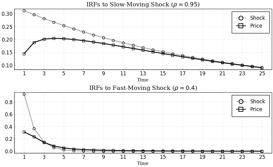

Lower Cost of Attention: $\omega=0.1$

Get the IRFs:

T = 25; #length of IRFs
irfs_lω = irfs(sol_lω,T = T);
nothing #hide

Plot IRFs:

p1 = plot(1:T, [irfs_lω.x[1,1,:], irfs_lω.a[1,1,:]],
    title             = L"IRFs to Slow-Moving Shock ($\rho = 0.95$)",
    label             = ["Shock" "Price"],
    color             = [:darkgray :black],
    marker            = [:circle :square],
    markerstrokecolor = :match,
    markercolor       = false,
    markersize        = 6)
p2 = plot(1:T, [irfs_lω.x[2,2,:], irfs_lω.a[1,2,:]],
    title             = L"IRFs to Fast-Moving Shock ($\rho = 0.4$)",
    label             = ["Shock" "Price"],
    color             = [:darkgray :black],
    marker            = [:circle :square],
    markerstrokecolor = :match,
    markercolor       = false,
    markersize        = 6)
p = plot(p1,p2,
    layout     = (2,1),
    xlabel     = "Time",
    lw         = 2,
    xticks     = (1:2:T),
    xlim       = (0,T+1),
    fontfamily = "serif",
    legend     = :topright,
    legendfont = font(12),
    tickfont   = font(12),
    size       = (900,550),
    framestyle = :box)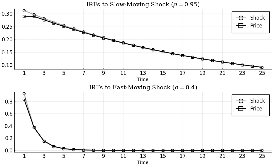

Other Discount Factors: $\beta\in\{0,1\}$

Get the IRFs:

T = 25; #length of IRFs
irfs_lβ = irfs(sol_lβ,T = T);
irfs_hβ = irfs(sol_hβ,T = T);
nothing #hide

Plot IRFs:

p1 = plot(1:T, [irfs_bp.x[1,1,:],irfs_hβ.a[1,1,:], irfs_lβ.a[1,1,:]],
    title             = L"IRFs to Slow-Moving Shock ($\rho = 0.95$)",
    label             = ["Shock" L"Price ($\beta=1$)" L"Price ($\beta=0$)"],
    color             = [:darkgray :black :gray50],
    marker            = [:circle :square :utriangle],
    markerstrokecolor = :match,
    markercolor       = false,
    markersize        = 6)
p2 = plot(1:T, [irfs_bp.x[2,2,:],irfs_hβ.a[1,2,:], irfs_lβ.a[1,2,:]],
    title             = L"IRFs to Fast-Moving Shock ($\rho = 0.4$)",
    label             = ["Shock" L"Priceblack ($\beta=1$)" L"Price ($\beta=0$)"],
    color             = [:darkgray :black :gray50],
    marker            = [:circle :square :utriangle],
    markerstrokecolor = :match,
    markercolor       = false,
    markersize        = 6)
p = plot(p1,p2,
    layout     = (2,1),
    xlabel     = "Time",
    lw         = 2,
    xticks     = (1:2:T),
    xlim       = (0,T+1),
    fontfamily = "serif",
    legend     = :topright,
    legendfont = font(12),
    tickfont   = font(12),
    size       = (900,550),
    framestyle = :box)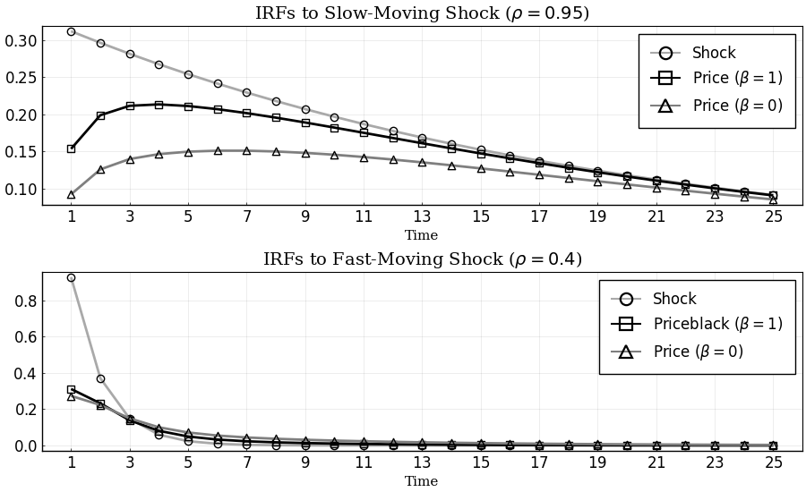

Extensions

Transition Dynamics of Attention

In this section, we solve for the transition dynamics of the optimal posterior covariance matrix starting from an initial prior that is different from the steady state prior.

For instance let us consider a case where the firm is at the steady state of the rational inattention problem at time 0, with prior covariance matrix $\bar{\Sigma}_{-1}$, and it receives a one time treatment with a perfectly informative signal about its optimal price:

\[s_0 = \mathbf{H}'\vec{x}_0\]

Solve for the transition dynamics

The function Trip solves for the transition dynamics automatically given the initial signal. Start by initializing the initial signal:

s0 = DRIPs.Signal(H,0.0);
nothing #hide

Solve for the transition dynamics given $s_0$:

Tss     = 15; # guess for time until convergence
bp_trip = Trip(sol_bp, s0; T = Tss);
nothing #hide

Performance for solving the transition dynamics for a random signal:

@benchmark Trip(sol_bp, S; T = 30) setup = (S = DRIPs.Signal(rand(2),0.0))

BenchmarkTools.Trial: 
  memory estimate:  501.02 KiB
  allocs estimate:  6200
  --------------
  minimum time:     487.478 μs (0.00% GC)
  median time:      519.538 μs (0.00% GC)
  mean time:        589.391 μs (10.83% GC)
  maximum time:     7.933 ms (87.83% GC)
  --------------
  samples:          8470
  evals/sample:     1

Plot Transition Path of Eigenvalues

Plot the marginal values of information. In this problem the state is two dimensional. At any time, for every orthogonalized dimension, the agent weighs the marginal value of acquiring information in that dimension against the marginal cost of attention which is the parameter $\omega$.The number of signals that the agent acquires at any time is the number of marginal values that are larger than $\omega$.

p = plot(0:Tss-1,[bp_trip.Ds[1,1:Tss],bp_trip.Ds[2,1:Tss],bp_trip.p.ω*ones(Tss,1)],
    label             = ["Low marginal value dim." "High marginal value dim." "Marginal cost of attention"],
    size              = (900,275),
    title             = "Marginal Value of Information",
    xlabel            = "Time",
    color             = [:darkgray :black :black],
    line              = [:solid :solid :dash],
    marker            = [:circle :square :none],
    markercolor       = false,
    markerstrokecolor = :match,
    markersize        = 6,
    xlim              = (-1,Tss),
    xticks            = 0:2:Tss-1,
    legend            = :outertopright,
    fontfamily        = "serif",
    framestyle        = :box)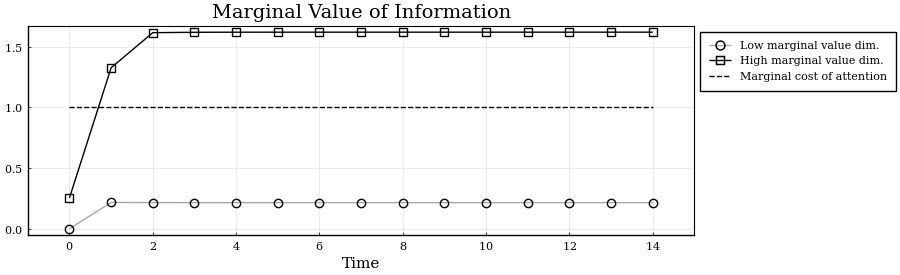

Impulse Response Functions with Information Treatment

Get the IRFs in the transition path after treatment:

T = 30;

tirfs_bp = irfs(sol_bp,s0,T = T); # irfs with treatment
irfs_bp  = irfs(sol_bp,T = T);    # irfs in the Ss (without treatment)
nothing #hide

Plot IRFs:

p1 = plot(1:T, [irfs_bp.x[1,1,:], tirfs_bp.a[1,1,:], irfs_bp.a[1,1,:]],
    title             = L"IRFs to Slow-Moving Shock ($\rho = 0.95$)",
    label             = ["Shock" "Price (w/ treatment)" "Price (w/o treatment)"],
    color             = [:darkgray :black :gray80],
    marker            = [:circle :square :utriangle],
    markerstrokecolor = :match,
    markercolor       = false,
    markersize        = 6)
p2 = plot(1:T, [tirfs_bp.x[2,2,:], tirfs_bp.a[1,2,:], irfs_bp.a[1,2,:]],
    title             = L"IRFs to Fast-Moving Shock ($\rho = 0.4$)",
    label             = ["Shock" "Price (w/ treatment)" "Price (w/o treatment)"],
    color             = [:darkgray :black :gray80],
    marker            = [:circle :square :utriangle],
    markerstrokecolor = :match,
    markercolor       = false,
    markersize        = 6)
p = plot(p1,p2,
    layout     = (2,1),
    xlabel     = "Time",
    lw         = 2,
    xticks     = (1:2:T),
    xlim       = (0,T+1),
    fontfamily = "serif",
    legend     = :topright,
    legendfont = font(12),
    tickfont   = font(12),
    size       = (900,550),
    framestyle = :box)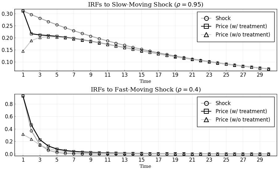

This page was generated using Literate.jl.